by R. Grothmann
In this notebook, we compute the total resistance of an electrical circuit.
As a first example, we assume a curcuit of type:
A - B - C - D, B - D
where each connection "-" has 1 Ohm resistance.
We like to know the resistance between A and D.
>shortformat;
First we set up the incidence matrix. This matrix has 1 on A[i,j] if i - j.
>A=[0,1,0,0;1,0,1,1;0,1,0,1;0,1,1,0]
        0         1         0         0
        1         0         1         1
        0         1         0         1
        0         1         1         0
The resistance problem is solved by assuming the flow through each knot is 0. The flow from i to j is (u[i]-u[j])*A[i,j], where u is the potential in i,j. Thus u must satisfy B.u=0 with the following matrix.
>B=A; B=setdiag(B,0,-sum(B)')
       -1         1         0         0
        1        -3         1         1
        0         1        -2         1
        0         1         1        -2
Additionally, we want u[1]=1, u[4]=-1.
>B[1]=0; B[1,1]=1; ...
 B[4]=0; B[4,4]=1; ...
 B
        1         0         0         0
        1        -3         1         1
        0         1        -2         1
        0         0         0         1
We can then compute the potentials u.
>fracformat; ...
 u=B\[1;0;0;-1]
                  1
               -1/5
               -3/5
                 -1
And the flow away from the first knot.
>f=sum(A[1])*u[1]-A[1].u
6/5
The total resistance is the total difference in potential 2 divided by the flow from the first knot.
>2/f
5/3
I have put these computations into an Euler file.
>load "incidence.e"
Functions to create incidence matix for a graph, and
to solve resistance potential in a graph. For a demo
load the Resitance.en notebook.
For more information use "help incidence.e" or see the
user menu.
>shortformat;
Define a matrix of connections and resistances. Each row contains the indices of two knots and the resistance of the connection between them.
>K=[1,2,1;2,3,1;2,4,1;3,4,1]
        1         2         1
        2         3         1
        2         4         1
        3         4         1
Make the incidence matrix.
>A=makeIncidence(K,4)
        0         1         0         0
        1         0         1         1
        0         1         0         1
        0         1         1         0
And solve the problem.
>fracformat; {u,r}=solvePotential(A,1,4); r, shortformat;
5/3
Here is a classical parallel circuit.
>K=[1,2,1;1,2,2;1,2,3]; {u,r}=solvePotential(makeIncidence(K,2),1,2); r,
0.545455
This is the same as we get with the well known formula.
>1/(1+1/2+1/3)
0.545455
Now a circuit with resistances in row.
>K=[1,2,1;2,3,2;3,4,3]; {u,r}=solvePotential(makeIncidence(K,4),1,4); r,
6
In this case, the resistances add.
>1+2+3
6
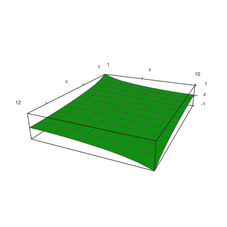
In the Euler file, there is a function to generate the incidence matrix of a rectangle grid. We solve the potential from one corner to the opposite.
>n=10; m=12;
>{u,r}=solvePotential(makeRectangleIncidence(n,m),1,n*m); r,
3.1579
Let us plot this potential.
>plot3d(1:m,(1:n)',redim(u,n,m),user=1,scale=1.3):
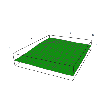
For two inner knots, the image looks like this.
>n0=floor(n/2); m0=floor(m/2);
>{u,r}=solvePotential(makeRectangleIncidence(n,m),(n0-2)*m+m0-1,n0*m+m0+1); r,
0.888949
>plot3d(1:m,(1:n)',redim(u,n,m),user=1,scale=1.3):
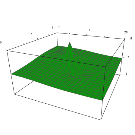
Now a large grid. Note, that the incidence matrix of these 400=20^2 points contains 400^2 elements.
>n=20; m=20;
>n0=floor(n/2); m0=floor(m/2);
>{u,r}=solvePotential(makeRectangleIncidence(n,m),(n0-2)*m+m0-1,n0*m+m0+1); r,
0.859987
>plot3d(1:m,(1:n)',redim(u,n,m)*5,scale=1.3):
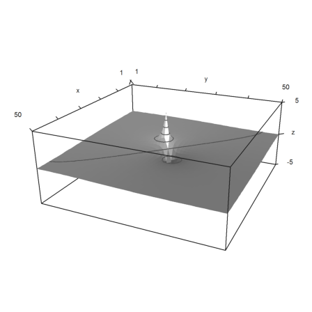
For really large problems, there is the Gauß-Seidel algorithm which was invented for such problems.
The following matrix would have 2500 unknowns in 2500 equations. But it is very thin with only about 5000 entries. So we store it in a compressed way.
>n=50; m=50;
>RX=makeRectangleX(n,m);
>n0=floor(n/2); m0=floor(m/2);
Now we solve with the conjugate gradient method for thin matrices (cgxfit). The solution takes a few seconds on a 2.0 GHz computer.
>{u,r}=solvePotentialX(RX,(n0-2)*m+m0-1,n0*m+m0+1); r,
0.850583
>plot3d(1:m,(1:n)',redim(u,n,m)*5,scale=[1,1,2],>contour, ...
   levels="thin",zoom=3.2):
We now take a very specific grid looking like this.
o - o - o - o - ... - o
| | | |
o - o - o - o - ... - o
The horizontal connections all have resistance 1 Ohm and the vertical given resistances v[1],...,v[n].
In the first example all v[i] are 1. We compute the resistance from left to right recursively.
>longformat; computeChain(ones(1,100))
0.732050807569
Of course the recursion in this example is
1/R[i] = 1/v[i] + 1/(2+R[i+1])
R[n] = v[n]
We can easily find the limit, if it exists, and see that n=100 is very close to this limit.
>&solve(1/x=1+1/(2+x),x); &float(%)
[x = - 2.732050807568877, x = 0.73205080756888]
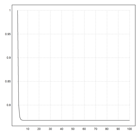
Let us increase the resistance by 1 from left to right.
>computeChain(1:100)
0.767563799989
To see the convergence, we define a function depending on n, and plot it.
>function test (n) := computeChain(1:n)
>plot2d(testmap(1:100)):
Some more examples.
>computeChain(1/(1:100))
0.706778468235
>computeChain(1/2^(1:100))
0.408209882798